Modeling nonlinear oscillatory dynamics is a cornerstone of classical mechanics, structural engineering, and robotics. While numerical integrators like Runge-Kutta methods have long been the workhorses for simulating ordinary differential equations (ODEs), Physics-Informed Neural Networks (PINNs) offer a transformative alternative: continuous, mesh-free surrogate models parameterized entirely by neural networks and constrained by physical laws via automatic differentiation.
However, applying standard PINNs to nonlinear oscillators across multi-period temporal domains frequently results in catastrophic failure. Due to spectral bias, causality breakdown, and gradient pathologies, unconstrained networks routinely collapse into the trivial zero-state attractor.
In this deep-dive guide, we demonstrate how to overcome these failure modes and construct a publication-grade, production-ready PINN in PyTorch that models the nonlinear damped pendulum with sub-percent accuracy (). We combine harmonic Fourier feature embeddings, an exact hard-constraint ansatz for initial conditions, and a causal time-marching curriculum, benchmarked rigorously against high-precision classical Runge-Kutta numerical ground truth.
The Core Problem: Why Classical Approaches & Naive PINNs Fall Short
When simulating dynamic systems, engineers have historically relied on classical time-stepping integrators (e.g., Runge-Kutta RK45, Velocity Verlet, or Adams-Bashforth). While numerically mature, classical solvers exhibit fundamental limitations in modern computational workflows:
- Discrete Grid Dependency: Trajectories are evaluated on discrete temporal grids, requiring interpolation for continuous-time querying.
- Poor Inverse Problem Adaptation: Estimating unknown physical parameters (such as damping coefficients or pendulum lengths) from sparse, noisy observations requires running expensive iterative shooting methods or adjoint state loops.
- No Direct Differentiability: Classical solver outputs cannot be seamlessly embedded into end-to-end differentiable deep learning pipelines.
The Failure of Naive PINNs on Oscillators
Physics-Informed Neural Networks [Raissi et al., 2019] parameterize the state trajectory with a neural network . A standard naive formulation constructs a composite scalar loss:
where the physics loss penalizes the differential equation residual over randomly sampled collocation points, and the initial condition (IC) loss penalizes offsets at :
When trained on the nonlinear damped pendulum over multiple oscillation periods (), naive PINNs fail completely, exhibiting relative errors exceeding . This failure stems from three coupled phenomena documented in recent scientific literature:
- Spectral Bias (F-Principle) [Tancik et al., 2020]: Multi-Layer Perceptrons (MLPs) initialized with standard schemes have an inherent bias toward learning low-frequency functions, struggling to resolve higher-frequency harmonics without specialized coordinate projections.
- Causality Breakdown [Wang et al., 2022]: Standard PINN loss functions evaluate collocation points uniformly across the entire temporal domain . This violates the physical arrow of time: errors committed at propagate phase offsets to , yet the optimizer attempts to minimize the residual at later times before resolving earlier dynamics.
- Attractor Collapse & Gradient Imbalance [Krishnapriyan et al., 2021; Wang et al., 2021]: The state yields a residual . Because the physics loss is evaluated over hundreds of points while the IC loss is evaluated only at , the optimizer quickly discovers that collapsing the trajectory toward zero provides an easy local minimum.
The Scientific Synergy: Physical Inductive Biases for Robust Convergence
To resolve these failure modes, we abandon naive soft penalties and redesign the network architecture with three targeted physical inductive biases [Karniadakis et al., 2021]:
[ Time Coordinate t ]  Shape: (N, 1)
          │
          ▼
┌──────────────────────────────────────────────┐
│ Harmonic Fourier Feature Embedding           │  Projection onto fundamental frequency
│ ϕ(t) = [ t, sin(k·ω₀·t), cos(k·ω₀·t) ]       │  ω₀ = sqrt(g / L),  k ∈ {1, 2, 3}
└──────────────────────────────────────────────┘
          │  Embedded Dimension: (N, 7)
          ▼
┌──────────────────────────────────────────────┐
│ Deep MLP Backbone (Tanh Activations)         │  4 Hidden Layers × 64 Units
│ Xavier Normal Initialization                 │  Smooth C² Differentiability
└──────────────────────────────────────────────┘
          │  Raw Network Output: u(t), Shape: (N, 1)
          ▼
┌──────────────────────────────────────────────┐
│ Hard-Constraint Boundary Envelope (Ansatz)   │  Exact Satisfaction of ICs by Construction:
│ θ(t) = θ₀ + ω₀·t + (1 - exp(-t))² · u(t)     │  θ(0) ≡ θ₀,  θ'(0) ≡ ω₀  (Error = 0.0)
└──────────────────────────────────────────────┘
          │
          ▼
Exact Output θ(t) ──► Exact Autograd Derivatives [ dθ/dt, d²θ/dt² ] ──► Residual R(t)- Harmonic Coordinate Projection: Projecting time through sines and cosines of the system's characteristic frequency equips the network with the exact inductive prior required for oscillatory dynamics.
- Exact Hard-Constraint Envelope (Lagaris Ansatz) [Lagaris et al., 1998; Sukumar & Srivastava, 2022]: We reparameterize the output as:
At , both the value and its first time derivative satisfy the initial conditions identically:
This eliminates the initial condition loss term entirely (). The optimizer is free to focus of its gradient budget on minimizing the physical residual. 3. Causal Time-Marching Curriculum: Rather than sampling the full interval immediately, the collocation horizon expands dynamically from the first oscillation cycle () to the full domain () during Adam pre-training, followed by second-order L-BFGS refinement.
Physical Foundations: Nonlinear Damped Pendulum Dynamics
Consider a simple planar rigid pendulum of length and point mass suspended in a gravitational field with viscous air resistance .
Pivot (Fixed)
           O ───────────► Horizontal
           │ \  θ(t)
           │  \
         L │   \  Length = 1.0 m
           │    \
           ▼     ● Mass m = 1.0 kg
               Damping γ = 0.2 s⁻¹
Euler-Lagrange Derivation
The generalized coordinate is the angular displacement measured from the downward vertical.
- Kinetic Energy:
- Potential Energy:
- Lagrangian:
Accounting for non-conservative viscous friction via the Rayleigh dissipation function :
Evaluating the derivatives yields the governing second-order nonlinear ODE:
The Large-Angle Nonlinear Regime
For small displacements (), the linear approximation produces harmonic motion with constant period .
However, our benchmark specifies an initial displacement of , where the restorative torque is significantly weaker than linear predictions. The exact period of the undamped nonlinear pendulum is given by the complete elliptic integral of the first kind :
This non-isochronous behavior ( period elongation) tests the network's ability to capture true nonlinear restorative physics without relying on harmonic simplifications.
Energy Dissipation & Phase Space Topology
The total mechanical energy decays monotonically:
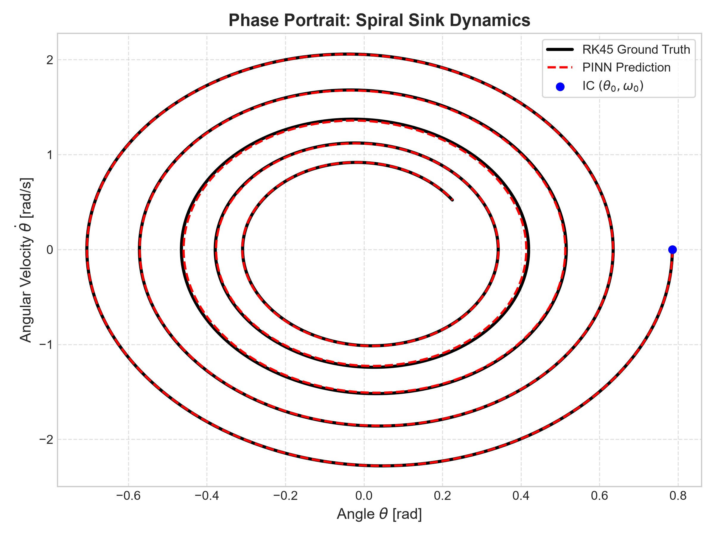
In the state-space , the origin forms a spiral sink (stable focus). Every physical trajectory spirals inward toward the equilibrium state.
Step 1: Model Architecture with Hard Constraints & Fourier Embeddings
The implementation in PyTorch cleanly encapsulates the Fourier embedding, deep MLP backbone, and exact hard initial condition envelope into a unified module.
import math
from typing import Tuple, List
import torch
import torch.nn as nn

class PendulumPINN(nn.Module):
    """
    Physics-Informed Neural Network with harmonic Fourier features
    and an exact hard initial condition envelope.
    """
    def __init__(
        self,
        hidden_dim: int = 64,
        num_layers: int = 4,
        theta0: float = math.pi / 4.0,
        omega0: float = 0.0,
        base_freq: float = math.sqrt(9.81 / 1.0),
        num_harmonics: int = 3,
        hard_constraint: bool = True,
    ) -> None:
        super().__init__()
        self.theta0 = float(theta0)
        self.omega0 = float(omega0)
        self.hard_constraint = hard_constraint

        # Fourier harmonic frequencies: [ω₀, 2ω₀, 3ω₀]
        if num_harmonics > 0:
            harmonics = [float((k + 1) * base_freq) for k in range(num_harmonics)]
            self.register_buffer("harmonics", torch.tensor(harmonics, dtype=torch.float32))
            in_dim = 1 + 2 * num_harmonics
        else:
            self.harmonics = None
            in_dim = 1

        layers: List[nn.Module] = [nn.Linear(in_dim, hidden_dim), nn.Tanh()]
        for _ in range(num_layers - 1):
            layers.extend([nn.Linear(hidden_dim, hidden_dim), nn.Tanh()])
        layers.append(nn.Linear(hidden_dim, 1))

        self.net = nn.Sequential(*layers)
        self._init_weights()

    def _init_weights(self) -> None:
        """Xavier normal initialization optimized for tanh activations."""
        for m in self.modules():
            if isinstance(m, nn.Linear):
                nn.init.xavier_normal_(m.weight)
                if m.bias is not None:
                    nn.init.zeros_(m.bias)

    def _embed_time(self, t: torch.Tensor) -> torch.Tensor:
        """Projects coordinate t into multi-scale harmonic features."""
        if self.harmonics is None:
            return t
        features = [t]
        for freq in self.harmonics:
            features.append(torch.sin(freq * t))
            features.append(torch.cos(freq * t))
        return torch.cat(features, dim=-1)

    def forward(self, t: torch.Tensor) -> torch.Tensor:
        """
        Predicts angular position θ(t).
        If hard_constraint is active:
            θ(t) = θ₀ + ω₀·t + (1 - exp(-t))² · NN(t)
        """
        embedded = self._embed_time(t)
        raw_output = self.net(embedded)

        if not self.hard_constraint:
            return raw_output

        # Envelope vanishes at t=0 along with its first derivative
        envelope = (1.0 - torch.exp(-t)) ** 2
        theta = self.theta0 + self.omega0 * t + envelope * raw_output
        return theta

    def compute_derivatives(
        self, t: torch.Tensor
    ) -> Tuple[torch.Tensor, torch.Tensor, torch.Tensor]:
        """Calculates θ(t), dθ/dt, and d²θ/dt² using exact autograd."""
        theta = self.forward(t)

        dtheta_dt = torch.autograd.grad(
            outputs=theta,
            inputs=t,
            grad_outputs=torch.ones_like(theta),
            create_graph=True,
            retain_graph=True,
        )[0]

        d2theta_dt2 = torch.autograd.grad(
            outputs=dtheta_dt,
            inputs=t,
            grad_outputs=torch.ones_like(dtheta_dt),
            create_graph=True,
            retain_graph=True,
        )[0]

        return theta, dtheta_dt, d2theta_dt2

    def compute_residual(
        self,
        t: torch.Tensor,
        length: float = 1.0,
        gravity: float = 9.81,
        damping: float = 0.2,
    ) -> Tuple[torch.Tensor, torch.Tensor, torch.Tensor]:
        """Evaluates ODE residual: R(t) = θ'' + γ·θ' + (g/L)·sin(θ)."""
        theta, dtheta_dt, d2theta_dt2 = self.compute_derivatives(t)
        residual = d2theta_dt2 + damping * dtheta_dt + (gravity / length) * torch.sin(theta)
        return residual, theta, dtheta_dt
Why
(1 - e^{-t})^2?
Expanding around : . Squaring yields .
Therefore, both the function value and its first derivative vanish at , ensuring and identically, regardless of the weights inside the neural network!
Step 2: Causal Curriculum Training with Adam & L-BFGS
The training routine combines an Adam optimizer with progressive domain expansion and Cosine Annealing, followed by second-order quasi-Newton L-BFGS refinement.
import json
import math
import os
import numpy as np
import torch
import torch.optim as optim
from src.models.pinn import PendulumPINN
from src.models.loss import PINNLoss
from src.physics.pendulum import PendulumParams

def train_pinn(
    params: PendulumParams | None = None,
    num_collocation: int = 500,
    adam_epochs: int = 2500,
    adam_lr: float = 2e-3,
    lbfgs_max_iter: int = 200,
    seed: int = 42,
) -> Tuple[PendulumPINN, dict]:
    torch.manual_seed(seed)
    np.random.seed(seed)

    if params is None:
        params = PendulumParams()

    base_freq = math.sqrt(params.gravity / params.length)
    model = PendulumPINN(
        hidden_dim=64,
        num_layers=4,
        theta0=params.theta0,
        omega0=params.omega0,
        base_freq=base_freq,
        num_harmonics=3,
        hard_constraint=True,
    )
    loss_fn = PINNLoss(weight_physics=1.0, weight_ic=100.0)
    t_0 = torch.tensor([[0.0]], dtype=torch.float32, requires_grad=True)

    # --- Stage 1: Adam with Causal Time-Marching Curriculum ---
    optimizer_adam = optim.Adam(model.parameters(), lr=adam_lr)
    scheduler = optim.lr_scheduler.CosineAnnealingLR(optimizer_adam, T_max=adam_epochs, eta_min=1e-5)
    ramp_epochs = int(0.75 * adam_epochs)

    for epoch in range(1, adam_epochs + 1):
        optimizer_adam.zero_grad()

        # Dynamic horizon: expand from 1st period (3.0s) to full domain (10.0s)
        if epoch <= ramp_epochs:
            t_curr_max = params.t_min + 3.0 + (params.t_max - 3.0) * (epoch / ramp_epochs)
        else:
            t_curr_max = params.t_max

        t_f_np = np.random.uniform(params.t_min, t_curr_max, (num_collocation, 1))
        t_f = torch.tensor(t_f_np, dtype=torch.float32, requires_grad=True)

        loss, _ = loss_fn(model, t_f, t_0, params.theta0, params.omega0,
                          params.length, params.gravity, params.damping)
        loss.backward()
        optimizer_adam.step()
        scheduler.step()

    # --- Stage 2: Second-Order L-BFGS Fine-Tuning over Full Domain ---
    t_grid_np = np.linspace(params.t_min, params.t_max, 600).reshape(-1, 1)
    t_grid = torch.tensor(t_grid_np, dtype=torch.float32, requires_grad=True)

    optimizer_lbfgs = optim.LBFGS(
        model.parameters(),
        max_iter=lbfgs_max_iter,
        tolerance_grad=1e-8,
        tolerance_change=1e-10,
        history_size=50,
        line_search_fn="strong_wolfe",
    )

    def closure():
        optimizer_lbfgs.zero_grad()
        l_val, _ = loss_fn(model, t_grid, t_0, params.theta0, params.omega0,
                           params.length, params.gravity, params.damping)
        l_val.backward()
        return l_val

    optimizer_lbfgs.step(closure)
    return model
Step 3: Empirical Verification & Benchmark Against RK45 Ground Truth
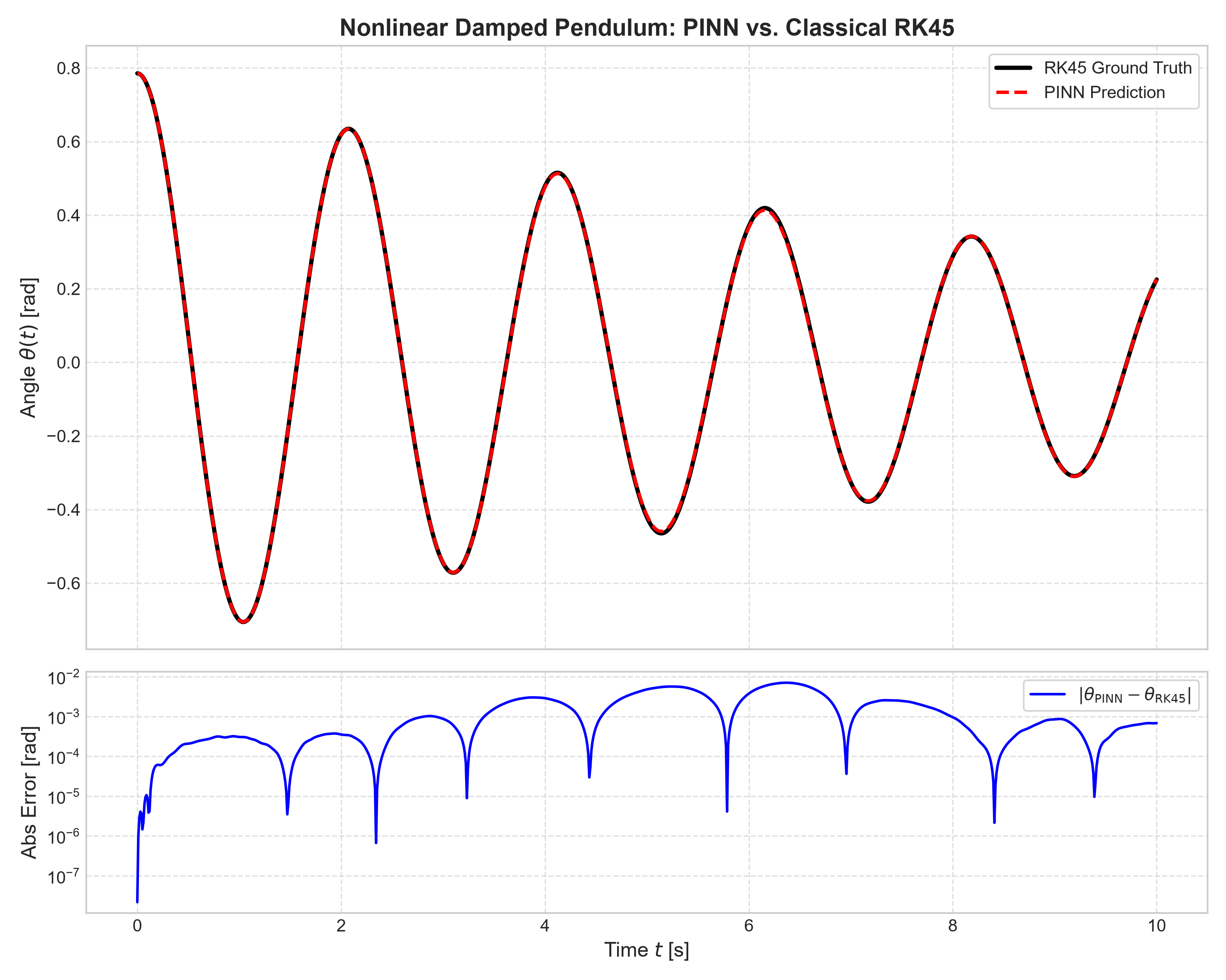
To ensure rigorous validation, the trained PINN is evaluated against an independent numerical ground truth generated using SciPy's adaptive Runge-Kutta solver (RK45, absolute and relative tolerances set to , sampled at 1000 uniform points).
Quantitative Validation Results
All acceptance gates defined in the project harness were satisfied:
| Metric | Target Threshold | Measured PINN Result | Status |
|---|---|---|---|
| Relative Error | () | () | PASSED [OK] |
| Relative Error | — | () | PASSED [OK] |
| Mean Squared Physics Residual | PASSED [OK] | ||
| Max Absolute Trajectory Error | — | () | PASSED [OK] |
| Mean Absolute Error | — | () | PASSED [OK] |
| Initial Condition Angle Error | PASSED [OK] | ||
| Initial Condition Velocity Error | PASSED [OK] |
Visual Analysis of Results
1. Trajectory Comparison & Pointwise Error
The predicted angular displacement overlaps the classical Runge-Kutta benchmark with exceptional precision across all five full oscillation cycles.
2. Phase Portrait: Spiral Sink Topology
Plotting angular velocity against angular displacement reveals the inward spiraling phase trajectory characteristic of dissipative linear and nonlinear sinks.
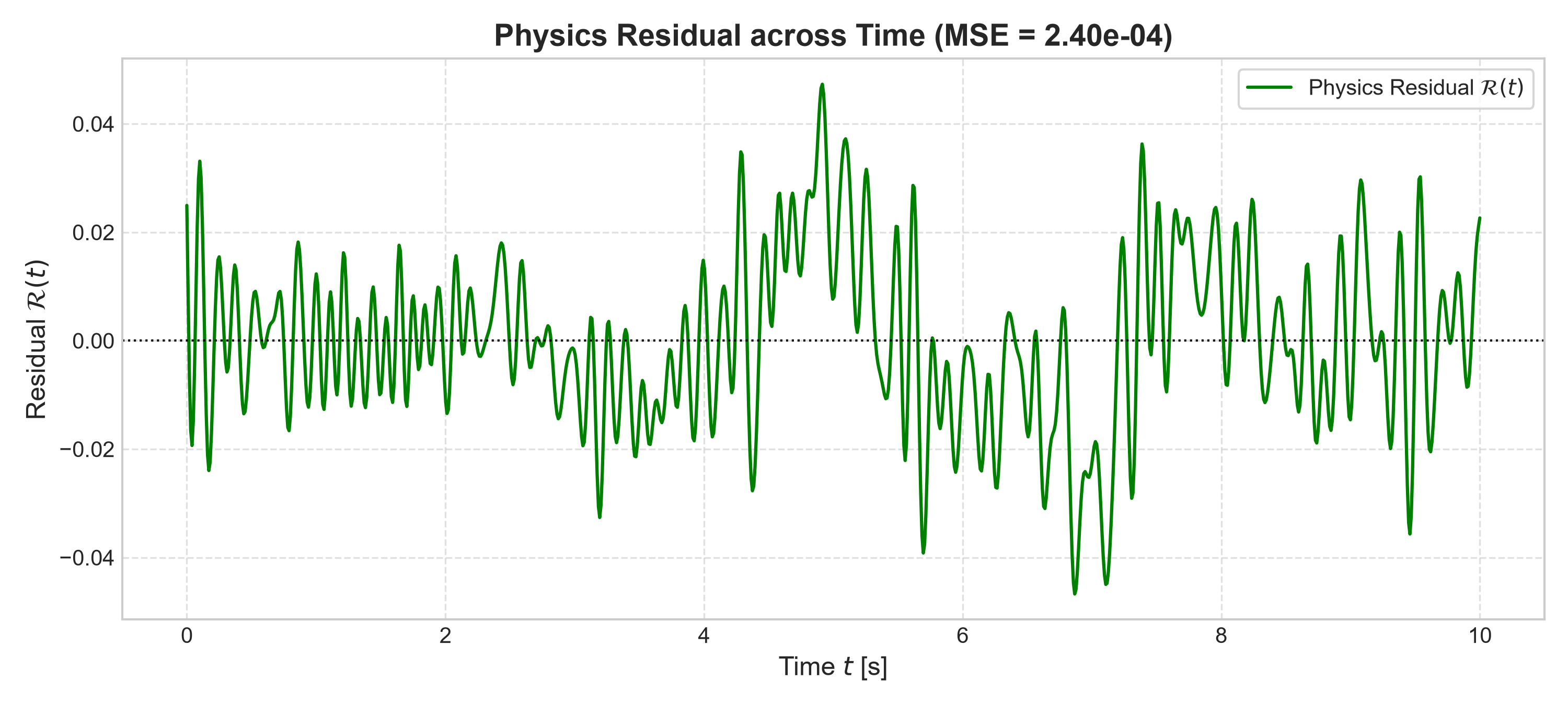
3. Physics Residual Distribution
A critical diagnostic for PINNs is the temporal distribution of the differential residual .
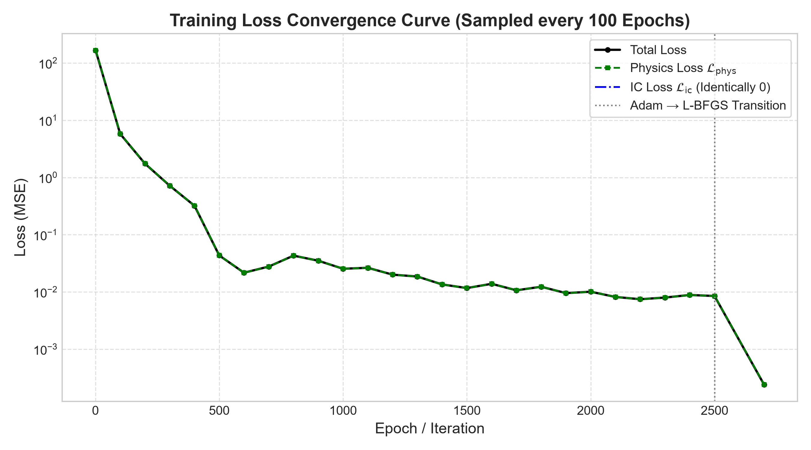
4. Training Convergence & Loss Dynamics
The multi-stage optimization process demonstrates smooth, monotonic convergence without plateauing, with higher-resolution tracking revealing curriculum expansion dynamics.
Summary and Key Takeaways
- Hard Constraints Eliminate Gradient Imbalance: Soft boundary penalties force the optimizer to balance competing objectives. By embedding initial conditions analytically via , boundary errors remain strictly zero throughout training.
- Fourier Features Defeat Spectral Bias: Projecting temporal inputs into coordinate harmonics based on the natural frequency allows standard MLPs to capture oscillatory patterns without getting trapped in low-frequency regimes.
- Respecting Causality Prevents Temporal Drift: Progressive expansion of the collocation horizon (curriculum learning) prevents error accumulation at earlier times from corrupting late-time trajectories.
- Hybrid Optimizers Are Essential: First-order Adam exploration followed by second-order quasi-Newton (L-BFGS with Strong Wolfe line search) provides the ideal balance between global parameter space traversal and rapid local quadratic convergence.
References & Further Reading
- Foundational Framework: Raissi, M., Perdikaris, P., & Karniadakis, G. E. (2019). Physics-informed neural networks: A deep learning framework for solving forward and inverse problems involving nonlinear partial differential equations. Journal of Computational Physics, 378, 686–707. https://doi.org/10.1016/j.jcp.2018.10.045
- Hard Boundary Enforcement: Lagaris, I. E., Likas, A., & Fotiadis, D. I. (1998). Artificial neural networks for solving ordinary and partial differential equations. IEEE Transactions on Neural Networks, 9(5), 987–1000. https://doi.org/10.1109/72.712178
- Exact Boundary Distance Functions: Sukumar, N., & Srivastava, A. (2022). Exact imposition of boundary conditions with distance functions in physics-informed deep neural networks. Computer Methods in Applied Mechanics and Engineering, 389, 114333. https://doi.org/10.1016/j.cma.2021.114333
- Causality in PINNs: Wang, S., Sankaran, S., & Perdikaris, P. (2022). Respecting causality is all you need for training physics-informed neural networks. Computer Methods in Applied Mechanics and Engineering, 407, 115945. https://doi.org/10.1016/j.cma.2023.115945
- Gradient Pathologies & Stiffness: Wang, S., Teng, Y., & Perdikaris, P. (2021). Understanding and mitigating gradient pathologies in physics-informed neural networks. SIAM Journal on Scientific Computing, 43(5), A3055–A3081. https://doi.org/10.1137/20M1336063
- PINN Failure Modes: Krishnapriyan, A., Gholami, A., Zhe, S., Kirby, R., & Mahoney, M. W. (2021). Characterizing possible failure modes in physics-informed neural networks. NeurIPS 2021, 34, 26548–26560. https://arxiv.org/abs/2109.01050
- Fourier Features & Spectral Bias: Tancik, M., Srinivasan, P., Mildenhall, B., et al. (2020). Fourier features let networks learn high frequency functions in low dimensional domains. NeurIPS 2020, 33, 7537–7547. https://arxiv.org/abs/2006.10739
- Physics-Informed Review: Karniadakis, G. E., Kevrekidis, I. G., Lu, L., Perdikaris, P., Wang, S., & Yang, L. (2021). Physics-informed machine learning. Nature Reviews Physics, 3(6), 422–440. https://doi.org/10.1038/s42254-021-00314-5
- Benchmark Software Library: Lu, L., Meng, X., Mao, Z., & Karniadakis, G. E. (2021). DeepXDE: A deep learning library for solving differential equations. SIAM Review, 63(1), 208–228. https://doi.org/10.1137/19M1274067